问题描述
在使用 R lme4 多级模型时,我正在努力计算连续预测变量的最大值-最小值之间的效应大小。
模拟数据:预测变量“x”的范围从 1 到 3
library(tidyverse)
n = 100
a = tibble(y = rep(c("pos","neg","neg"),length.out = n),x = rep(3,group = rep(letters[1:7],length.out = n))
b = tibble(y = rep(c("pos","pos",x = rep(2,length.out = n))
c = tibble(y = rep(c("pos",x = rep(1,length.out = n))
d = rbind(a,b)
df = rbind(d,c)
df = df %>% mutate(y = as.factor(y))
df

模型
library("lme4")
m = glmer(
  y ~ x + (x | group),data = df,family = binomial(link = "logit"))
输出
ggpredict(m,"x")
.
# Predicted probabilities of y

x | Predicted |       95% CI
----------------------------
1 |      0.75 | [0.67,0.82]
2 |      0.50 | [0.44,0.56]
3 |      0.25 | [0.18,0.33]

Adjusted for:
* group = 0 (population-level)
我无法计算预测变量的“x”最大值 (3) 和最小值 (1) 之间的效果大小
我最好的尝试
library("emmeans")
emmeans(m,"x",trans = "logit",type = "response",at = list(x = c(1,3)))
 x response     SE  df asymp.LCL asymp.UCL
 1     0.75 0.0387 Inf     0.667     0.818
 3     0.25 0.0387 Inf     0.182     0.333

Confidence level used: 0.95
Intervals are back-transformed from the logit scale
如何使用预测变量的“x”最大值 (3) 和最小值 (1) 之间的 CI 计算效果大小? 效果大小应该在概率范围内。
解决方法
我会尽力回答,尽管我仍然不确定问题是什么。我将假设需要的是两个概率之间的差异。
显示的 emmeans 调用中有很多活动部分,因此我将分步进行。首先,让我们估算一下相关概率:
> library(emmeans)
> EMM = emmeans(m,"x",at = list(x = c(1,3)),type = "response")
> EMM
 x prob     SE  df asymp.LCL asymp.UCL
 1 0.75 0.0387 Inf     0.667     0.818
 3 0.25 0.0387 Inf     0.182     0.333

Confidence level used: 0.95
Intervals are back-transformed from the logit scale
获得成对比较的最快方法是通过
> pairs(EMM)
 contrast odds.ratio   SE  df null z.ratio p.value
 1 / 3             9 2.94 Inf    1   6.728  <.0001

Tests are performed on the log odds ratio scale
如注释中所述(以及在文档中,例如 vignette on comparisons,当对数或 logit 转换到位时,比较显示为比率。发生这种情况是因为测试是在链接(logit)尺度,log之间的差异是一个比率的对数。
如果我们想要概率之间的差异,则有必要创建一个新对象,其中估计的主要数量是概率,而不是它们的对数。在emmeans中,这可以通过regrid()函数完成:
> EMMP = regrid(EMM,transform = "response")
> EMMP
 x prob     SE  df asymp.LCL asymp.UCL
 1 0.75 0.0387 Inf     0.674     0.826
 3 0.25 0.0387 Inf     0.174     0.326

Confidence level used: 0.95
这个输出看起来很像EMM的总结;然而,logit 转换的所有记忆都已被删除,因此置信区间是不同的,因为它们是直接从 prob 估计值的 SE 计算出来的。有关详细信息,请参阅 vignette on transformations。
所以现在如果我们比较这些,我们就会得到概率的差异:
> confint(pairs(EMMP))
 contrast estimate     SE  df asymp.LCL asymp.UCL
 1 - 3         0.5 0.0612 Inf      0.38      0.62

Confidence level used: 0.95
(注意:我将其包裹在 confint() 中,以便我们获得置信区间,而不是 t 比率的默认摘要和P 值。)
这可以在一行代码中完成,如下所示:
confint(pairs(emmeans(m,transform = "response",3)))))
transform 参数要求立即将参考网格传递给 regrid()。请注意,此处的正确参数是 transform = "response",而不是 transform = "logit"(即,指定要以什么结束,而不是从什么开始)。后者撤消,然后重做 logit 转换,让您回到起点。
emmeans 包提供了很多选项,我真的建议您阅读小插曲。
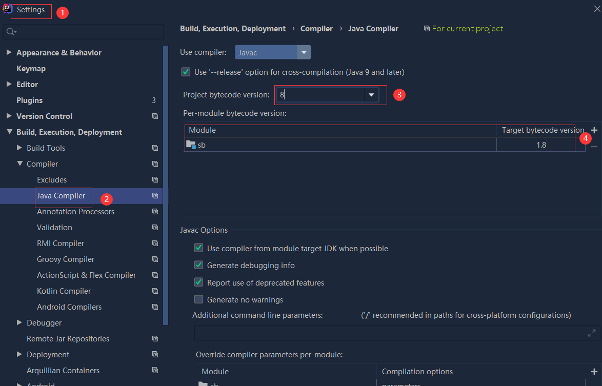 依赖报错 idea导入项目后依赖报错,解决方案:https://blog....
 错误1:gradle项目控制台输出为乱码 # 解决方案:https://bl...