Chapter 1
1. Selecting columns
counties %>%
  # Select the columns
  select(state, county, population, poverty)
2. Arranging observations
counties_selected <- counties %>%
  select(state, county, population, private_work, public_work, self_employed)

counties_selected %>%
  # Add a verb to sort in descending order of public_work
  arrange(desc(public_work))
3. Filtering for conditions
counties_selected <- counties %>%
  select(state, county, population)

counties_selected %>%
  # Filter for counties with a population above 1000000
  filter(state == "California", population > 1000000)
4. Mutate
counties_selected <- counties %>%
  select(state, county, population, public_work)

counties_selected %>%
  # Add a new column public_workers with the number of people employed in public work
  mutate(public_workers = population * public_work / 100) %>%
  # Sort in descending order of the public_workers column
  arrange(desc(public_workers))
5. Conclusion
counties %>%
  # Select the five columns
  select(state, county, population, men, women) %>%
  # Add the proportion_men variable
  mutate(proportion_men = men / population) %>%
  # Filter for population of at least 10,000
  filter(population >= 10000) %>%
  # Arrange proportion of men in descending order
  arrange(desc(proportion_men))
Chapter 2
1. The count verb
eg1. Use count() to find the number of counties in each region, using a second argument to sort in descending order.
# Use count to find the number of counties in each region
counties_selected %>%
  count(region, sort = TRUE)
eg2. Count the number of counties in each state, weighted based on the citizens column, and sorted in descending order.
# Find number of counties per state, weighted by citizens, sorted in descending order
counties_selected %>%
  count(state, wt = citizens, sort = TRUE)
2. The group by, summarize and ungroup verbs
eg1.
counties_selected %>%
  # Summarize to find minimum population, maximum unemployment, and average income
  summarize(min_population = min(population), max_unemployment = max(unemployment), average_income = mean(income))
eg2. Group the data by state, and summarize to create the columns total_area (with total area in square miles) and total_population (with total population).
counties_selected %>%
  # Group by state
  group_by(state) %>%
  # Find the total area and population
  summarize(total_area = sum(land_area), total_population = sum(population))
eg3. Add a density column with the people per square mile, then arrange in descending order.
counties_selected %>%
  group_by(state) %>%
  summarize(total_area = sum(land_area),
            total_population = sum(population)) %>%
  # Add a density column
  mutate(density = total_population / total_area) %>%
  # Sort by density in descending order
  arrange(desc(density))
eg4. Summarize to find the total population, as a column called total_pop, in each combination of region and state
counties_selected %>%
  # Group and summarize to find the total population
  group_by(region, state) %>%
  summarize(total_pop = sum(population))
eg5. Notice the tibble is still grouped by region; use another summarize() step to calculate two new columns: the average state population in each region (average_pop) and the median state population in each region (median_pop).
counties_selected %>%
  # Group and summarize to find the total population
  group_by(region, state) %>%
  summarize(total_pop = sum(population)) %>%
  # Calculate the average_pop and median_pop columns
  summarize(average_pop = mean(total_pop), median_pop = median(total_pop))
3. The top_n verb
counties_selected <- counties %>%
  select(region, state, county, metro, population, walk)
eg1. Find the county in each region with the highest percentage of citizens who walk to work.
counties_selected %>%
  # Group by region
  group_by(region) %>%
  # Find the greatest number of citizens who walk to work
  top_n(1,walk)
eg2. In how many states do more people live in metro areas than non-metro areas?
(Recall that the metro column has one of the two values "metro" (for high-density city areas) or "Nonmetro" (for suburban and country areas).)
counties_selected <- counties %>%
  select(state, metro, population)
counties_selected %>%
# Find the total population for each combination of state and metro
group_by(state, metro) %>%
summarize(total_pop = sum(population)) %>%
# Extract the most populated row for each state
top_n(1, total_pop) %>%
# Count the states with more people in Metro or Nonmetro areas
ungroup() %>%
count(metro)Chapter 3
1. Selecting
(1) colon( : )
...
$ professional       <dbl> 33.2, 33.1, 26.8, 21.5, 28.5, 18.8, 27.5, 27.3, 23.~
$ service            <dbl> 17.0, 17.7, 16.1, 17.9, 14.1, 15.0, 16.6, 17.7, 14.~
$ office             <dbl> 24.2, 27.1, 23.1, 17.8, 23.9, 19.7, 21.9, 24.2, 26.~
$ construction       <dbl> 8.6, 10.8, 10.8, 19.0, 13.5, 20.1, 10.3, 10.5, 11.5~
$ production         <dbl> 17.1, 11.2, 23.1, 23.7, 19.9, 26.4, 23.7, 20.4, 24.~
...
eg. Select the columns for state, county, population and (using a colon) all five of those industry-related variables; there are five consecutive variables in the table related to the industry of people's work: professional, service, office, construction, and production.
counties %>%
  # Select state, county, population, and industry-related columns
  select(state, county, population, professional:production) %>%
  # Arrange service in descending order
  arrange(desc(service))
(2) starts_with() / ends_with()
eg.
counties %>%
  # Select the state, county, population, and those ending with "work"
  select(state, county, population, ends_with("work")) %>%
  # Filter for counties that have at least 50% of people engaged in public work
  filter(public_work >= 50)
2. The rename verb
eg1.
counties %>%
  # Count the number of counties in each state
  count(state) %>%
  # Rename the n column to num_counties
  rename(num_counties = n)
eg2.
counties %>%
# Select state, county, and poverty as poverty_rate
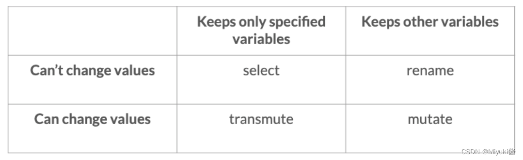
select(state, county, poverty_rate = poverty)3. The transmute verb
transmute: you can use to calculate new columns while dropping other columns
eg1. Keep only the state, county, and population columns, and add a new column, density, that contains the population per land_area.
counties %>%
  # Keep the state, county, and populations columns, and add a density column
  transmute(state, county, population, density = population / land_area)
eg2.
# Change the name of the unemployment column
counties %>%
  rename(unemployment_rate = unemployment)

# Keep the state and county columns, and the columns containing poverty
counties %>%
  select(state, county, contains("poverty"))

# Calculate the fraction_women column without dropping the other columns
counties %>%
  mutate(fraction_women = women / population)

# Keep only the state, county, and employment_rate columns
counties %>%
  transmute(state, county, employment_rate = employed / population)
Chapter 4
1. The babynames data
eg1. Filter for only the names Steven, Thomas, and Matthew, and assign it to an object called selected_names.
selected_names <- babynames %>%
  # Filter for the names Steven, Thomas, and Matthew
  filter(name %in% c("Steven", "Thomas", "Matthew"))
eg2. Visualize those three names as a line plot over time, with each name represented by a different color.
# Plot the names using a different color for each name
ggplot(selected_names, aes(x = year, y = number, color = name)) +
  geom_line()
2. Grouped mutates
eg1. calculate the total number of people born in that year in this dataset as year_total.
# Calculate the fraction of people born each year with the same name
babynames %>%
  group_by(year) %>%
  mutate(year_total = sum(number)) %>%
  ungroup() %>%
  mutate(fraction = number / year_total)
eg2. Now use your newly calculated fraction column, in combination with top_n(), to identify the year each name is most common,.
# Calculate the fraction of people born each year with the same name
babynames %>%
  group_by(year) %>%
  mutate(year_total = sum(number)) %>%
  ungroup() %>%
  mutate(fraction = number / year_total) %>%
  # Find the year each name is most common
  group_by(name) %>%
  top_n(1, fraction)
eg3. Use a grouped mutate to add two columns: (1) name_total, with the sum of the number of babies born with that name in the entire dataset. (2) name_max, with the maximum number of babies born in any year.
babynames %>%
  # Add columns name_total and name_max for each name
  group_by(name) %>%
  mutate(name_total = sum(number), name_max = max(number))
eg4. (1) Add another step to ungroup the table. (2) Add a column called fraction_max containing the number in the year divided by name_max.
babynames %>%
  # Add columns name_total and name_max for each name
  group_by(name) %>%
  mutate(name_total = sum(number),
         name_max = max(number)) %>%
  # Ungroup the table
  ungroup() %>%
  # Add the fraction_max column containing the number by the name maximum
  mutate(fraction_max = number / name_max)
3. Window functions
v <- c(1, 3, 6, 14)
v
# 输出结果
[1] 1 3 6 14

lag(v)
# 输出结果
[1] NA 1 3 6

v - lag(v)
# 输出结果
[1] NA 2 3 8
eg. (1) Arrange the data in ascending order of name and then year. (2) Group by name so that your mutate works within each name. (3) Add a column ratio containing the ratio (not difference) of fraction between each year.
babynames_fraction %>%
  # Arrange the data in order of name, then year
  arrange(name, year) %>%
  # Group the data by name
  group_by(name) %>%
  # Add a ratio column that contains the ratio of fraction between each year
  mutate(ratio = fraction / lag(fraction))