Alink漫谈(十五) :多层感知机 之 迭代优化
0x00 摘要
Alink 是阿里巴巴基于实时计算引擎 Flink 研发的新一代机器学习算法平台,是业界首个同时支持批式算法、流式算法的机器学习平台。本文和前文将带领大家来分析Alink中多层感知机的实现。
因为Alink的公开资料太少,所以以下均为自行揣测,肯定会有疏漏错误,希望大家指出,我会在日后随时更新。
0x01 前文回顾
从前文 ALink漫谈(十四) :多层感知机 之 总体架构 我们了解了多层感知机的概念以及Alink中的整体架构,下面我们就要开始介绍如何优化。
1.1 基本概念
我们再次温习下基本概念:
-
神经元输入:类似于线性回归 z = w1x1+ w2x2 +⋯ + wnxn = wT・x(linear threshold unit (LTU))。
-
神经元输出:激活函数,类似于二值分类,模拟了生物学中神经元只有激发和抑制两种状态。增加偏值,输出层哪个节点权重大,输出哪一个。
-
采用Hebb准则,下一个权重调整方法参考当前权重和训练效果。
-
如何自动化学习计算权重——backpropagation,即首先正向做一个计算,根据当前输出做一个error计算,作为指导信号反向调整前一层输出权重使其落入一个合理区间,反复这样调整到第一层,每轮调整都有一个学习率,调整结束后,网络越来越合理。
1.2 误差反向传播算法
基于误差反向传播算法(backpropagation,BP)的前馈神经网络训练过程可以分为以下三步:
- 在前向传播时计算每一层的净输入z(l)和激活值a(l),直至最后一层;
- (反向传播阶段)将激励响应同训练输入对应的目标输出求差,从而获得隐层和输出层的响应误差。用误差反向传播计算每一层的误差项 δ(l);
- 对于每个突触上的权重,按照以下步骤进行更新:将输入激励和响应误差相乘,从而获得权重的梯度;将这个梯度乘上一个比例并取反后加到权重上。即计算每一层参数的偏导数,并更新参数。
这个比例(百分比)将会影响到训练过程的速度和效果,因此称为”训练因子”。梯度的方向指明了误差扩大的方向,因此在更新权重的时候需要对其取反,从而减小权重引起的误差。
1.3 总体逻辑
我们回顾下总体逻辑。
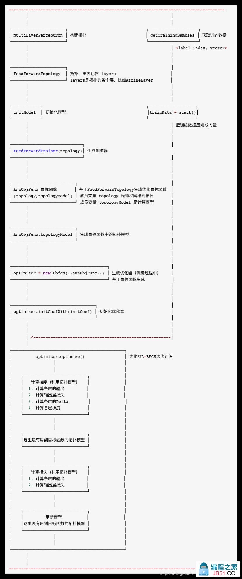
0x02 训练神经网络
这部分是重头戏,所以要从总体逻辑中剥离出来单独说。
FeedForwardTrainer.train 函数会完成神经网络的训练,即:
DataSet<DenseVector> weights = trainer.train(trainData,getParams());
其逻辑大致如下:
- 1)初始化模型
initCoef = initModel(data,this.topology); - 2)把训练数据压缩成向量,
trainData = stack()。这里应该是为了减少传输数据量。需要注意,其把输入数据从二元组<label index,vector>转换为三元组Tuple3.of((double) count,0.,stacked); - 3)生成优化目标函数
new AnnObjFunc(topology...) - 4)构建训练器
FeedForwardTrainer - 5)训练器会基于目标函数构建优化器
Optimizer optimizer = new Lbfgs,即使用L-BFGS来训练神经网络;
2.1 初始化模型
初始化模型相关代码如下:
DataSet<DenseVector> initCoef = initModel(data,this.topology); // 随机初始化权重系数
optimizer.initCoefWith(initCoef);

public void initCoefWith(DataSet<DenseVector> initCoef) {
	this.coefVec = initCoef; // 就是赋值在内部变量上
}
这里需要和线性回归比较下:
-
线性回归中,假如有两个特征,则初始系数为
coef = {DenseVector} "0.001 0.0 0.0 0.0",4个数值具体是"权重,b,w1,w2"。 -
多层感知机这里,初始化系数则是一个
DenseVector。
initModel 主要就是随机初始化权重系数。精华函数在 topology.getWeightSize() 部分。
private DataSet<DenseVector> initModel(DataSet<?> inputRel,final Topology topology) {
        if (initialWeights != null) {
          ......
        } else {
            return BatchOperator.getExecutionEnvironmentFromDataSets(inputRel).fromElements(0)
                .map(new RichMapFunction<Integer,DenseVector>() {
                    ......
                    @Override
                    public DenseVector map(Integer value) throws Exception {
                        // 这里是精华,获取了系数的size
                        DenseVector weights = DenseVector.zeros(topology.getWeightSize());

                        for (int i = 0; i < weights.size(); i++) {
                            weights.set(i,random.nextGaussian() * initStdev);//随机初始化
                        }
                        return weights;
                    }
                })
                .name("init_weights");
        }
}
topology.getWeightSize() 调用的是 FeedForwardTopology的函数,就是遍历各层,累加求系数和。
@Override
public int getWeightSize() {
        int s = 0;
        for (Layer layer : layers) { //遍历各层
            s += layer.getWeightSize();
        }
        return s;
}
AffineLayer系数大小如下:
@Override
public int getWeightSize() {
		return numIn * numOut + numOut;
}
FuntionalLayer 没有系数
@Override
public int getWeightSize() {
	return 0;
}
SoftmaxLayerWithCrossEntropyLoss 没有系数
@Override
public int getWeightSize() {
	return 0;
}
回顾本例对应拓扑:
this = {FeedForwardTopology@4951}
 layers = {ArrayList@4944}  size = 4
      0 = {AffineLayer@4947} // 仿射层
       numIn = 4
       numOut = 5
      1 = {FuntionalLayer@4948}
       activationFunction = {SigmoidFunction@4953}  // 激活函数
      2 = {AffineLayer@4949} // 仿射层
       numIn = 5
       numOut = 3
      3 = {SoftmaxLayerWithCrossEntropyLoss@4950}  // 激活函数
所以最后 DenseVector 向量大小是两个仿射层的和(4 + 5 * 5)+ (5 + 3 * 3) = 43。
2.2 压缩数据
这里把输入数据二元组 <label index,vector> 转换,压缩到 DenseVector中。这里压缩的目的应该是为了减少传输数据量。
如果输入是:
batchData = {ArrayList@11527}  size = 64
 0 = {Tuple2@11536} "(2.0,6.5 2.8 4.6 1.5)"
  f0 = {Double@11572} 2.0
  f1 = {DenseVector@11573} "6.5 2.8 4.6 1.5"
 1 = {Tuple2@11537} "(1.0,6.1 3.0 4.9 1.8)"
  f0 = {Double@11575} 1.0
  f1 = {DenseVector@11576} "6.1 3.0 4.9 1.8"
.....
则最终输出的压缩数据是:
batch = {Tuple3@11532}
 f0 = {Double@11578} 18.0
 f1 = {Double@11579} 0.0
 f2 = {DenseVector@11580} "6.5 2.8 4.6 1.5 6.1 3.0 4.9 1.8 7.3 2.9 6.3 1.8 5.7 2.8 4.5 1.3 6.4 2.8 5.6 2.1 6.7 2.5 5.8 1.8 6.3 3.3 4.7 1.6 7.2 3.6 6.1 2.5 7.2 3.0 5.8 1.6 4.9 2.4 3.3 1.0 7.4 2.8 6.1 1.9 6.5 3.2 5.1 2.0 6.6 2.9 4.6 1.3 7.9 3.8 6.4 2.0 5.2 2.7 3.9 1.4 6.4 2.7 5.3 1.9 6.8 3.0 5.5 2.1 5.7 2.5 5.0 2.0 2.0 1.0 1.0 2.0 1.0 1.0 2.0 1.0 1.0 2.0 1.0 1.0 2.0 1.0 2.0 1.0 1.0 1.0"
具体代码如下:
static DataSet<Tuple3<Double,Double,Vector>>
    stack(DataSet<Tuple2<Double,DenseVector>> data ...) {

        return data
            .mapPartition(new MapPartitionFunction<Tuple2<Double,DenseVector>,Tuple3<Double,Vector>>() {
                @Override
                public void mapPartition(Iterable<Tuple2<Double,DenseVector>> samples,Collector<Tuple3<Double,Vector>> out) throws Exception {
                    List<Tuple2<Double,DenseVector>> batchData = new ArrayList<>(batchSize);
                    int cnt = 0;
                    Stacker stacker = new Stacker(inputSize,outputSize,onehot);
                    for (Tuple2<Double,DenseVector> sample : samples) {
                        batchData.set(cnt,sample);
                        cnt++;
                        if (cnt >= batchSize) { // 如果已经大于默认的数据块大小,就直接发送
                            // 把batchData的x-vec压缩到DenseVector中
                            Tuple3<Double,Vector> batch = stacker.stack(batchData,cnt);
                            out.collect(batch);
                            cnt = 0;
                        }
                    }

                    // 如果压缩成功,则输出
                    if (cnt > 0) { // 没有大于默认数据块大小,也发送。cnt就是目前的数据块大小,针对本实例,是19,这也是后面能看到 matrix 维度 19 的来源。
                        Tuple3<Double,cnt);
                        out.collect(batch);
                    }
                }
            })
            .name("stack_data");
}
2.3 生成优化目标函数
回顾关于损失函数和目标函数的说明:
- 损失函数:计算的是一个样本的误差;
- 代价函数:是整个训练集上所有样本误差的平均,经常和损失函数混用;
- 目标函数:代价函数 + 正则化项;
多层感知机中生成目标函数代码如下:
final AnnObjFunc annObjFunc = new AnnObjFunc(topology,inputSize,onehotLabel,optimizationParams);
AnnObjFuncs是多层感知机优化的目标函数,其定义如下:
- topology 就是神经网络的拓扑;
- stacker 是用来压缩解压(后续L-BFGS是向量操作,所以也需要从矩阵到向量来回转换);
- topologyModel 是计算模型;
我们可以看到,在 AnnObjFunc 的 API 中调用时候,会看 AnnObjFunc.topologyModel 是否有值,如果没有就生成。
public class AnnObjFunc extends OptimObjFunc {
    private Topology topology;
    private Stacker stacker;
    private transient TopologyModel topologyModel = null;

    @Override
    protected double calcLoss(Tuple3<Double,Vector> labledVector,DenseVector coefVector) {
        // 看 AnnObjFunc.topologyModel 是否有值,如果没有就生成
        if (topologyModel == null) {
            topologyModel = topology.getModel(coefVector);
        } else {
            topologyModel.resetModel(coefVector);
        }
        Tuple2<DenseMatrix,DenseMatrix> unstacked = stacker.unstack(labledVector);
        return topologyModel.computeGradient(unstacked.f0,unstacked.f1,null);
    }

    @Override
    protected void updateGradient(Tuple3<Double,DenseVector coefVector,DenseVector updateGrad) {
        // 看 AnnObjFunc.topologyModel 是否有值,如果没有就生成
        if (topologyModel == null) {
            topologyModel = topology.getModel(coefVector);
        } else {
            topologyModel.resetModel(coefVector);
        }
        Tuple2<DenseMatrix,DenseMatrix> unstacked = stacker.unstack(labledVector);
        topologyModel.computeGradient(unstacked.f0,updateGrad);
    }
}
2.4 生成目标函数中的拓扑模型
如上所述,这个具体生成是在 AnnObjFunc 的 API 中调用时候,会看 AnnObjFunc.topologyModel 是否有值,如果没有就生成。这里会根据 FeedForwardTopology 的 layers 来生成拓扑模型。
public TopologyModel getModel(DenseVector weights) {
	FeedForwardModel feedForwardModel = new FeedForwardModel(this.layers);
	feedForwardModel.resetModel(weights);
	return feedForwardModel;
}
拓扑模型定义如下,能够看到里面有具体层 & 层模型。
public class FeedForwardModel extends TopologyModel {
    private List<Layer> layers; //具体层
    private List<LayerModel> layerModels; //层模型
    /**
     * Buffers of outputs of each layers.
     */
    private transient List<DenseMatrix> outputs = null;
    /**
     * Buffers of deltas of each layers.
     */
    private transient List<DenseMatrix> deltas = null;

    public FeedForwardModel(List<Layer> layers) {
        this.layers = layers;
        this.layerModels = new ArrayList<>(layers.size());
        for (int i = 0; i < layers.size(); i++) {
            layerModels.add(layers.get(i).createModel());
        }
    }
}
优化函数是根据每一层来建立模型,比如
public LayerModel createModel() {
	return new AffineLayerModel(this);
}
下面就看看具体各层模型的状况。
2.4.1 AffineLayerModel
定义如下,其具体函数比如 eval,computePrevDelta,grad 我们后续会提及。
public class AffineLayerModel extends LayerModel {
    private DenseMatrix w;
    private DenseVector b;

    // buffer for holding gradw and gradb
    private DenseMatrix gradw;
    private DenseVector gradb;

    private transient DenseVector ones = null;
}
2.4.2 FuntionalLayerModel
定义如下,其具体函数比如 eval,computePrevDelta,grad 我们后续会提及。
public class FuntionalLayerModel extends LayerModel {
    private FuntionalLayer layer;
}
2.4.3 SoftmaxLayerModelWithCrossEntropyLoss
这个就是针对最终输出层。
SoftmaxWithLoss层包含softmax和求交叉熵两部分。
对于softmax的输入向量 z,其输出向量的第 k 个值为:
而交叉熵损失函数:
损失函数对 a 求导,可得到:
具体代码如下,基本就是数学公式的实现。
public class SoftmaxLayerModelWithCrossEntropyLoss extends LayerModel
    implements AnnLossFunction {
    @Override
    public double loss(DenseMatrix output,DenseMatrix target,DenseMatrix delta) {
        int batchSize = output.numRows();
        MatVecOp.apply(output,target,delta,(o,t) -> t * Math.log(o));
        double loss = -(1.0 / batchSize) * delta.sum();
        MatVecOp.apply(output,t) -> o - t);
        return loss;
    }
}
2.4.3 最终模型
最终的模型如下:
this = {FeedForwardModel@10575}

     layers = {ArrayList@10576}  size = 4
          0 = {AffineLayer@10601}
          1 = {FuntionalLayer@10335}
          2 = {AffineLayer@10602}
          3 = {SoftmaxLayerWithCrossEntropyLoss@10603}

     layerModels = {ArrayList@10579}  size = 4
          0 = {AffineLayerModel@10581}
          1 = {FuntionalLayerModel@10433}
          2 = {AffineLayerModel@10582}
          3 = {SoftmaxLayerModelWithCrossEntropyLoss@10583}

     outputs = null
     deltas = null
用图形化简要表示如下(FeedForwardModel中省略了层):

2.5 生成优化器
回顾下概念。
针对目标函数最普通的优化是穷举法,对各个可能的权值遍历,找寻使损失最小的一组,但是这种方法会陷入嵌套循环里,使得运行速率大打折扣,于是就有了优化器。优化器的目的使快速找到目标函数最优解。
损失函数的目的是在训练过程中找到最合适的一组权值序列,也就是让损失函数降到尽可能低。优化器或优化算法用于将损失函数最小化,在每个训练周期或每轮后更新权重和偏置值,直到损失函数达到全局最优。
我们要寻找损失函数的最小值,首先一定有一个初始的权值,伴随一个计算得出来的损失。那么我们要想到损失函数最低点,要考虑两点:往哪个方向前进;前进多少距离。
因为我们想让损失值下降得最快,肯定是要找当前损失值在损失函数的切线方向,这样走最快。如果是在三维的损失函数上面,则更加明显,三维平面上的点做切线会产生无数个方向,而梯度就是函数在某个点无数个变化的方向中变化最快的那个方向,也就是斜率最大的那个方向。梯度是有方向的,负梯度方向就是下降最快的方向。
那么梯度下降是怎么运行的呢,刚才我们找到了逆梯度方向来作为我们前进的方向,接下来只需要解决走多远的问题。于是我们引入学习率,我们要走的距离就是梯度的大小*学习率。因为越优化梯度会越小,因此移动的距离也会越来越短。学习率的设置不能太大,否则可能会跳过最低点而导致梯度爆炸或者梯度消失;也不能设置太小,否则梯度下降可能十分缓慢。
优化算法有两种:
-
一阶优化算法。这些算法使用与参数相关的梯度值最小化或最大化代价函数。一阶导数告诉我们函数是在某一点上递减还是递增,简而言之,它给出了与曲面切线。
-
二阶优化算法。这些算法使用二阶导数来最小化代价函数,也称为Hessian。由于二阶导数的计算成本很高,所以不常使用二阶导数。二阶导数告诉我们一阶导数是递增的还是递减的,这表示了函数的曲率。二阶导数为我们提供了一个与误差曲面曲率相接触的二次曲面。
多层感知机这里使用L-BFGS优化器 来训练神经网络。
Optimizer optimizer = new Lbfgs(
            data.getExecutionEnvironment().fromElements(annObjFunc),trainData,BatchOperator
                .getExecutionEnvironmentFromDataSets(data)
                .fromElements(inputSize),optimizationParams
        );
optimizer.initCoefWith(initCoef);
0x03 L-BFGS训练
这部分又比较复杂,需要单独拿出来说,就是用优化器来训练。
optimizer.optimize()
  .map(new MapFunction<Tuple2<DenseVector,double[]>,DenseVector>() {
    @Override
    public DenseVector map(Tuple2<DenseVector,double[]> value) throws Exception {
        return value.f0;
    }
});
关于 L-BFGS 的细节,可以参见前面文章。 Alink漫谈(十一) :线性回归 之 L-BFGS优化 。
这里把 Lbfgs 类拿出来概要说明:
public class Lbfgs extends Optimizer {
    public DataSet <Tuple2 <DenseVector,double[]>> optimize() {
       DataSet <Row> model = new IterativeComQueue()
           ......
          .add(new CalcGradient())
           ......
          .add(new CalDirection(...))
          .add(new CalcLosses(...))
           ......
          .add(new UpdateModel(...))
           ......
          .exec();
    }
}
能够看到其中几个关键步骤:
-
CalcGradient()计算梯度 -
CalDirection(...)计算方向 -
CalcLosses(...)计算损失 -
UpdateModel(...)更新模型
算法框架都是基本不变的,所差别的就是具体目标函数和损失函数的不同。比如线性回归采用的是UnaryLossObjFunc,损失函数是 SquareLossFunc。
我们把多层感知机特殊之处填充关键步骤,得到与线性回归的区别。
-
CalcGradient()计算梯度- 1)调用
AnnObjFunc.updateGradient;- 1.1)调用 目标函数中拓扑模型
topologyModel.computeGradient来计算- 1.1.1)计算各层的输出;
forward(data,true) - 1.1.2)计算输出层损失;
labelWithError.loss - 1.1.3)计算各层的Delta;
layerModels.get(i).computePrevDelta - 1.1.4)计算各层梯度;`layerModels.get(i).grad
- 1.1.1)计算各层的输出;
- 1.1)调用 目标函数中拓扑模型
- 1)调用
-
CalDirection(...)计算方向- 这里的实现没有用到目标函数的拓扑模型。
-
CalcLosses(...)计算损失- 1)调用
AnnObjFunc.updateGradient;- 1.1)调用 目标函数中拓扑模型
topologyModel.computeGradient来计算- 1.1.1)计算各层的输出;
forward(data,true) - 1.1.2)计算输出层损失;
labelWithError.loss
- 1.1.1)计算各层的输出;
- 1.1)调用 目标函数中拓扑模型
- 1)调用
-
UpdateModel(...)更新模型- 这里的实现没有用到目标函数的拓扑模型。
3.1 CalcGradient 计算梯度
CalcGradient.calc 函数中会调用到目标函数的计算梯度功能。
// calculate local gradient
Double weightSum = objFunc.calcGradient(labledVectors,coef,grad.f0);
objFunc.calcGradient函数就是基类 OptimObjFunc 的实现,此处才会调用到 AnnObjFunc.updateGradient 的具体实现。
updateGradient(labelVector,coefVector,grad);
3.1.1 目标函数
回顾目标函数定义:
public class AnnObjFunc extends OptimObjFunc {

    protected void updateGradient(Tuple3<Double,DenseVector updateGrad) {
        if (topologyModel == null) {
            topologyModel = topology.getModel(coefVector);
        } else {
            topologyModel.resetModel(coefVector);
        }
        Tuple2<DenseMatrix,updateGrad);
    }
}
-
首先是生成拓扑模型;这步骤已经在前面提到了。
-
然后是
unstacked = stacker.unstack(labledVector);,解压数据,返回return Tuple2.of(features,labels);。 -
最后就是计算梯度;这是
FeedForwardModel类实现的。
3.1.2 计算梯度
计算梯度(此函数也负责计算损失)代码在 FeedForwardModel.computeGradient,大致逻辑如下:
CalcGradient.calc 会调用 objFunc.calcGradient(OptimObjFunc 的实现)
- 1)调用
AnnObjFunc.updateGradient;- 1.1)调用 目标函数中拓扑模型
topologyModel.computeGradient来计算- 1.1.1)计算各层的输出;
forward(data,true) - 1.1.2)计算输出层损失;
labelWithError.loss - 1.1.3)计算各层的Delta;
layerModels.get(i).computePrevDelta - 1.1.4)计算各层梯度;`layerModels.get(i).grad
- 1.1.1)计算各层的输出;
- 1.1)调用 目标函数中拓扑模型
代码如下:
public double computeGradient(DenseMatrix data,DenseVector cumGrad) {
        // data 是 x,target是y
        // 计算各层的输出
        outputs = forward(data,true);

        int currentBatchSize = data.numRows();
        if (deltas == null || deltas.get(0).numRows() != currentBatchSize) {
            deltas = new ArrayList<>(layers.size() - 1);
            int inputSize = data.numCols();
            for (int i = 0; i < layers.size() - 1; i++) {
                int outputSize = layers.get(i).getOutputSize(inputSize);
                deltas.add(new DenseMatrix(currentBatchSize,outputSize));
                inputSize = outputSize;
            }
        }
        int L = layerModels.size() - 1;
        AnnLossFunction labelWithError = (AnnLossFunction) this.layerModels.get(L);
        // 计算损失
        double loss = labelWithError.loss(outputs.get(L),deltas.get(L - 1));
        if (cumGrad == null) {
            return loss; // 如果只计算损失,则直接返回。
        }
        // 计算Delta;
        for (int i = L - 1; i >= 1; i--) {
            layerModels.get(i).computePrevDelta(deltas.get(i),outputs.get(i),deltas.get(i - 1));
        }
        int offset = 0;
        // 计算梯度;
        for (int i = 0; i < layerModels.size(); i++) {
            DenseMatrix input = i == 0 ? data : outputs.get(i - 1);
            if (i == layerModels.size() - 1) {
                layerModels.get(i).grad(null,input,cumGrad,offset);
            } else {
                layerModels.get(i).grad(deltas.get(i),offset);
            }
            offset += layers.get(i).getWeightSize();
        }
        return loss;
}
3.1.2.1 计算各层的输出
回忆下示例代码,我们设置神经网络是:
.setLayers(new int[]{4,5,3})
具体说就是调用各层模型的 eval 函数,其中第一层不好写入循环,所以单独写出。
public class FeedForwardModel extends TopologyModel {
    public List<DenseMatrix> forward(DenseMatrix data,boolean includeLastLayer) {
        .....
        layerModels.get(0).eval(data,outputs.get(0));
        int end = includeLastLayer ? layers.size() : layers.size() - 1;
        for (int i = 1; i < end; i++) {
            layerModels.get(i).eval(outputs.get(i - 1),outputs.get(i));
        }
        return outputs;
	}
}
具体各层调用如下:
AffineLayerModel.eval
这就是简单的仿射变换 WX + b,然后放入output。其中
@Override
public void eval(DenseMatrix data,DenseMatrix output) {
        int batchSize = data.numRows();
        for (int i = 0; i < batchSize; i++) {
            for (int j = 0; j < this.b.size(); j++) {
                output.set(i,j,this.b.get(j));
            }
        }
        BLAS.gemm(1.,data,false,this.w,1.,output);
}
其中 w,b 都是预置的。
this = {AffineLayerModel@10581}
 w = {DenseMatrix@10592} "mat[4,5]:\n  0.07807905200944776,-0.03040913035034301,.....\n"
 b = {DenseVector@10593} "-0.058043439717701296 0.1415366160323592 0.017773419483873353 -0.06802435221045448 0.022751460286303204"
 gradw = {DenseMatrix@10594} "mat[4,5]:\n  0.0,0.0,0.0\n  0.0,0.0\n"
 gradb = {DenseVector@10595} "0.0 0.0 0.0 0.0 0.0"
 ones = null
FuntionalLayerModel.eval
实现如下
public void eval(DenseMatrix data,DenseMatrix output) {
        for (int i = 0; i < data.numRows(); i++) {
            for (int j = 0; j < data.numCols(); j++) {
                output.set(i,this.layer.activationFunction.eval(data.get(i,j)));
            }
        }
}
类变量为
this = {FuntionalLayerModel@10433}
 layer = {FuntionalLayer@10335}
  activationFunction = {SigmoidFunction@10755}
输入是
data = {DenseMatrix@10642} "mat[19,5]:\n  0.09069152145840428,-0.4117319046979133,-0.273491600786707,-0.3638766081567865,-0.17552469317567304\n"
 m = 19
 n = 5
 data = {double[95]@10668}
其中,activationFunction 就调用到了 SigmoidFunction.eval。
public class SigmoidFunction implements ActivationFunction {
    @Override
    public double eval(double x) {
        return 1.0 / (1 + Math.exp(-x));
    }
}
SoftmaxLayerModelWithCrossEntropyLoss.eval
这里就是计算了最终输出。
    public void eval(DenseMatrix data,DenseMatrix output) {
        int batchSize = data.numRows();
        for (int ibatch = 0; ibatch < batchSize; ibatch++) {
            double max = -Double.MAX_VALUE;
            for (int i = 0; i < data.numCols(); i++) {
                double v = data.get(ibatch,i);
                if (v > max) {
                    max = v;
                }
            }
            double sum = 0.;
            for (int i = 0; i < data.numCols(); i++) {
                double res = Math.exp(data.get(ibatch,i) - max);
                output.set(ibatch,i,res);
                sum += res;
            }
            for (int i = 0; i < data.numCols(); i++) {
                double v = output.get(ibatch,i);
                output.set(ibatch,v / sum);
            }
        }
    }
3.1.2.2 计算损失
代码是:
AnnLossFunction labelWithError = (AnnLossFunction) this.layerModels.get(L);
double loss = labelWithError.loss(outputs.get(L),deltas.get(L - 1));
if (cumGrad == null) {
	return loss; // 可以直接返回
}
如果不需要计算梯度,则直接返回,否则继续进行。我们这里继续执行。
具体就是调用SoftmaxLayerModelWithCrossEntropyLoss的损失函数,就是输出层的损失。
output就是输出层,target就是label y。计算损失几乎和常规一样,只不过多了一个除以 batchSize。
public double loss(DenseMatrix output,t) -> o - t);
        return loss;
}
3.1.2.3 计算delta
梯度下降法需要计算损失函数对参数的偏导数,如果用链式法则对每个参数逐一求偏导,涉及到矩阵微分,效率比较低。所以在神经网络中经常使用反向传播算法来高效地计算梯度。具体就是在利用误差反向传播算法计算出每一层的误差项后,就可以得到每一层参数的梯度。
我们定义delta为隐含层的加权输入影响总误差的程度,即 delta_i 表示 第l层神经元的误差项,它用来表示第l层神经元对最终损失的影响,也反映了最终损失对第l层神经元的敏感程度。

上面这个公式就是误差的反向传播公式!因为第l层的误差项可以通过第l+1层的误差项计算得到。反向传播算法的含义是:第 l 层的一个神经元的误差项等于该神经元激活函数的梯度,再乘上所有与该神经元相连接的第l+1层的神经元的误差项的权重和。这里 W 是所有权重与偏置的集合)。
这个可能不好理解,找到三种解释,也许能够帮助大家增加理解:
- 因为梯度下降法是沿梯度(斜率)的反方向移动,所以我们往回倒,就要乘以梯度,再爬回去。
- 或者 可以看做错误(delta)的反向传递。经过一个线就乘以线的权重,经过点就乘以节点的偏导(sigmoid的偏导形式简洁)。
- 或者这么理解:输出层误差在转置权重矩阵的帮助下,传递到了隐藏层,这样我们就可以利用间接误差来更新与隐藏层相连的权重矩阵。权重矩阵在反向传播的过程中同样扮演着运输兵的作用,只不过这次是搬运的输出误差,而不是输入信号。
具体代码如下
for (int i = L - 1; i >= 1; i--) {
	layerModels.get(i).computePrevDelta(deltas.get(i),deltas.get(i - 1));
}
需要注意的是:
- 最后一层的delta已经在前一个loss计算出来,通过loss函数参数存储在 deltas.get(L - 1) 之中;
- 循环是从后数第二层向前计算;
本实例中,output是四层(03),deltas是三层(02)。
用output第4层的数值,来计算deltas第3层的数值。
用output第3层的数值 和 deltas第3层的数值,来计算deltas第2层的数值。具体细化到每层:
AffineLayerModel
public void computePrevDelta(DenseMatrix delta,DenseMatrix output,DenseMatrix prevDelta) {
	BLAS.gemm(1.0,true,prevDelta);
}
gemm函数作用是 C := alpha * A * B + beta * C . 这里可能是以为 b 小,就省略了计算。(存疑,如果有哪位朋友知道原因,请告知,谢谢)
public static void gemm(double alpha,DenseMatrix matA,boolean transA,DenseMatrix matB,boolean transB,double beta,DenseMatrix matC)
在这里是:1.0 * delta * this.w + 0 * prevDelta。delta 不转置,this.w 转置
FuntionalLayerModel
这里是 导数 * delta,导数就是变化率。
public void computePrevDelta(DenseMatrix delta,DenseMatrix prevDelta) {
        for (int i = 0; i < delta.numRows(); i++) {
            for (int j = 0; j < delta.numCols(); j++) {
                double y = output.get(i,j);
                prevDelta.set(i,this.layer.activationFunction.derivative(y) * delta.get(i,j));
            }
        }
}
激活函数是 The sigmoid function. f(x) = 1 / (1 + exp(-x)).
public class SigmoidFunction implements ActivationFunction {
    @Override
    public double eval(double x) {
        return 1.0 / (1 + Math.exp(-x));
    }

    @Override
    public double derivative(double z) {
        return (1 - z) * z; // 这里
    }
}
3.1.2.4 计算梯度
这里是从前往后计算,最后累计在cumGrad。
int offset = 0;
for (int i = 0; i < layerModels.size(); i++) {
    DenseMatrix input = i == 0 ? data : outputs.get(i - 1);
    if (i == layerModels.size() - 1) {
    	layerModels.get(i).grad(null,offset);
    } else {
    	layerModels.get(i).grad(deltas.get(i),offset);
    }
    offset += layers.get(i).getWeightSize();
}
AffineLayerModel
因为导数有两部分: w,所以这里有分为两部分计算。unpack 是为了解压缩,pack目的是最后L-BFGS是必须用向量来计算。
    public void grad(DenseMatrix delta,DenseMatrix input,DenseVector cumGrad,int offset) {
        unpack(cumGrad,offset,this.gradw,this.gradb);
        int batchSize = input.numRows();
        // 计算w
        BLAS.gemm(1.0,1.0,this.gradw);
        if (ones == null || ones.size() != batchSize) {
            ones = DenseVector.ones(batchSize);
        }
        // 计算b
        BLAS.gemv(1.0,this.ones,this.gradb);
        pack(cumGrad,this.gradb);
    }
FuntionalLayerModel
这里就没有梯度计算‘
public void grad(DenseMatrix delta,int offset) {}
最后类变量如下:
this = {FeedForwardModel@10394}

    layers = {ArrayList@10405}  size = 4
     0 = {AffineLayer@10539}
     1 = {FuntionalLayer@10377}
     2 = {AffineLayer@10540}
     3 = {SoftmaxLayerWithCrossEntropyLoss@10541}

    layerModels = {ArrayList@10401}  size = 4
     0 = {AffineLayerModel@10543}
     1 = {FuntionalLayerModel@10376}
     2 = {AffineLayerModel@10544}
     3 = {SoftmaxLayerModelWithCrossEntropyLoss@10398}

     outputs = {ArrayList@10399}  size = 4
      0 = {DenseMatrix@10374} "mat[19,5]:\n  0.5258035858891295,0.40832346939250874,0.4339942803542127,0.4146645474481978,0.45503123177429533..."
      1 = {DenseMatrix@10374} "mat[19,0.45503123177429533..."
      2 = {DenseMatrix@10533} "mat[19,3]:\n  0.31968260294191225,0.3305393733681367,0.3497780236899511..."
      3 = {DenseMatrix@10533} "mat[19,0.3497780236899511\...."

     deltas = {ArrayList@10400}  size = 3
      0 = {DenseMatrix@10375} "mat[19,5]:\n  0.0052001689807435756,-0.002841992490130668,0.02414893572802383."
      1 = {DenseMatrix@10379} "mat[19,5]:\n  0.02085622230356763,-0.011763437253154471,0.09830897540282763,-0.005205953747031061."
      2 = {DenseMatrix@10528} "mat[19,3]:\n  -0.6803173970580878,0.3497780236899511\."
3.2 CalDirection 计算方向
这里的实现没有用到目标函数的拓扑模型。
3.3 CalcLosses 计算损失
会在 objFunc.calcSearchValues 中就直接进入到了 AnnObjFunc 类内部。
计算损失代码如下:
for (Tuple3<Double,Vector> labelVector : labelVectors) {
    for (int i = 0; i < numStep + 1; ++i) {
		losses[i] += calcLoss(labelVector,stepVec[i]) * labelVector.f0;
    }
}
AnnObjFunc 的 calcLoss代码如下,可见是调用其拓扑模型来完成计算。
protected double calcLoss(Tuple3<Double,DenseVector coefVector) {
        if (topologyModel == null) {
            topologyModel = topology.getModel(coefVector);
        } else {
            topologyModel.resetModel(coefVector);
        }
        Tuple2<DenseMatrix,null);
}
这里调用的是 computeGradient 来计算损失,会提前返回
@Override
public double computeGradient(DenseMatrix data,DenseVector cumGrad) {
        outputs = forward(data,true);
        ......
        AnnLossFunction labelWithError = (AnnLossFunction) this.layerModels.get(L);
        double loss = labelWithError.loss(outputs.get(L),deltas.get(L - 1));
        if (cumGrad == null) {
            return loss; // 这里计算返回
        }
        ...
}
3.4 UpdateModel 更新模型
这里没有用到目标函数的拓扑模型。
0x04 输出模型
多层感知机比普通算法更耗费内存,我需要再IDEA中增加VM启动参数,才能运行成功。
-Xms256m -Xmx640m -XX:PermSize=128m -XX:MaxPermSize=512m
这里要小小吐槽一下Alink,在本地调试时候,没有办法修改Env的参数,比如心跳时间等。造成了调试的不方便。
输出模型算法如下:
        // output model
        DataSet<Row> modelRows = weights
            .flatMap(new RichFlatMapFunction<DenseVector,Row>() {
                @Override
                public void flatMap(DenseVector value,Collector<Row> out) throws Exception {
                    List<Tuple2<Long,Object>> bcLabels = getRuntimeContext().getBroadcastVariable("labels");
                    Object[] labels = new Object[bcLabels.size()];
                    bcLabels.forEach(t2 -> {
                        labels[t2.f0.intValue()] = t2.f1;
                    });

                    MlpcModelData model = new MlpcModelData(labelType);
                    model.labels = Arrays.asList(labels);
                    model.meta.set(ModelParamName.IS_VECTOR_INPUT,isVectorInput);
                    model.meta.set(MultilayerPerceptronTrainParams.LAYERS,layerSize);
                    model.meta.set(MultilayerPerceptronTrainParams.VECTOR_COL,vectorColName);
                    model.meta.set(MultilayerPerceptronTrainParams.FEATURE_COLS,featureColNames);
                    model.weights = value;
                    new MlpcModelDataConverter(labelType).save(model,out);
                }
            })
            .withBroadcastSet(labels,"labels");

// 当运行时候,参数如下:
value = {DenseVector@13212}
     data = {double[43]@13252}
      0 = -39.6567702949874
      1 = 16.74206842333768
      2 = 64.49084799006972
      3 = -1.6630682281137472
  ......
其中模型数据类定义如下
public class MlpcModelData {
    public Params meta = new Params();
    public DenseVector weights;
    public TypeInformation labelType;
    public List<Object> labels;
}
最终模型数据大致如下:
model = {Tuple3@13307} "
     f0 = {Params@13308} "Params {vectorCol=null,isVectorInput=false,layers=[4,3],featureCols=["sepal_length","sepal_width","petal_length","petal_width"]}"
      params = {HashMap@13326}  size = 4
       "vectorCol" -> null
       "isVectorInput" -> "false"
       "layers" -> "[4,3]"
       "featureCols" -> "["sepal_length","petal_width"]"
     f1 = {ArrayList@13309}  size = 1
      0 = "{"data":[-39.65676994108487,16.742068271166456,64.49084741971454,-1.6630682163468897,-66.71571933711216,-75.86297804171262,62.609759182998204,-101.47431688844591,31.546529394499977,17.597934397561986,85.36235323961661,-126.30772079054803,326.2329896163572,-29.720070636859894,-180.1693204840142,47.70255002863321,-63.44460914025362,136.6269589647343,-0.6446457887679123,-81.86976832863223,-16.333532816181705,15.4253068036318,-11.297177263474234,-1.1338164486683862,1.3011810728093451,-261.50388539155716,223.36901758842117,38.01966001651569,231.51463912615586,-152.59659885027318,-79.02863627644948,-48.28342595225583,-63.63975869014504,111.98667709535484,153.39174290331553,-121.04900950767653,-32.47876659498367,137.82909902591624,-43.99785013791728,-93.99354048054636,42.85135076273807,-24.8725999157641,-17.962438639217815]}"
       value = {char[829]@13325}
       hash = 0
     f2 = {Arrays$ArrayList@13310}  size = 3
      0 = "Iris-setosa"
      1 = "Iris-virginica"
      2 = "Iris-versicolor"
0xFF 参考
https://github.com/fengbingchun/NN_Test
[深度学习] [梯度下降]用代码一步步理解梯度下降和神经网络(ANN))
 文章浏览阅读5.3k次,点赞10次,收藏39次。本章详细写了mysq...
 文章浏览阅读1.8k次,点赞50次,收藏31次。本篇文章讲解Spar...
 文章浏览阅读928次,点赞27次,收藏18次。
 文章浏览阅读1.1k次,点赞24次,收藏24次。作用描述分布式协...
 文章浏览阅读1.5k次,点赞26次,收藏29次。为贯彻执行集团数...