英雄联盟胜负预测--简易肯德基上校

作为一名英雄联盟老玩家，巅峰时也曾打上过艾欧尼亚超凡大师，通过这关游戏让我认识了很多朋友，它也陪我度过了大部分校园青春。这是我第一次以学者的角度去面对它。

这里我们使用决策树ID3算法完成简易的英雄联盟胜负的预测。

AI遮天传 ML-决策树_老师我作业忘带了的博客-CSDN博客

 

第一步：战绩获取

首先呢我们可以进入英雄联盟官网，根据不同的游戏id爬取出这个赛季的详细战绩。

这里我们获取前10分钟的特征(因此不考虑纳什男爵等因素)

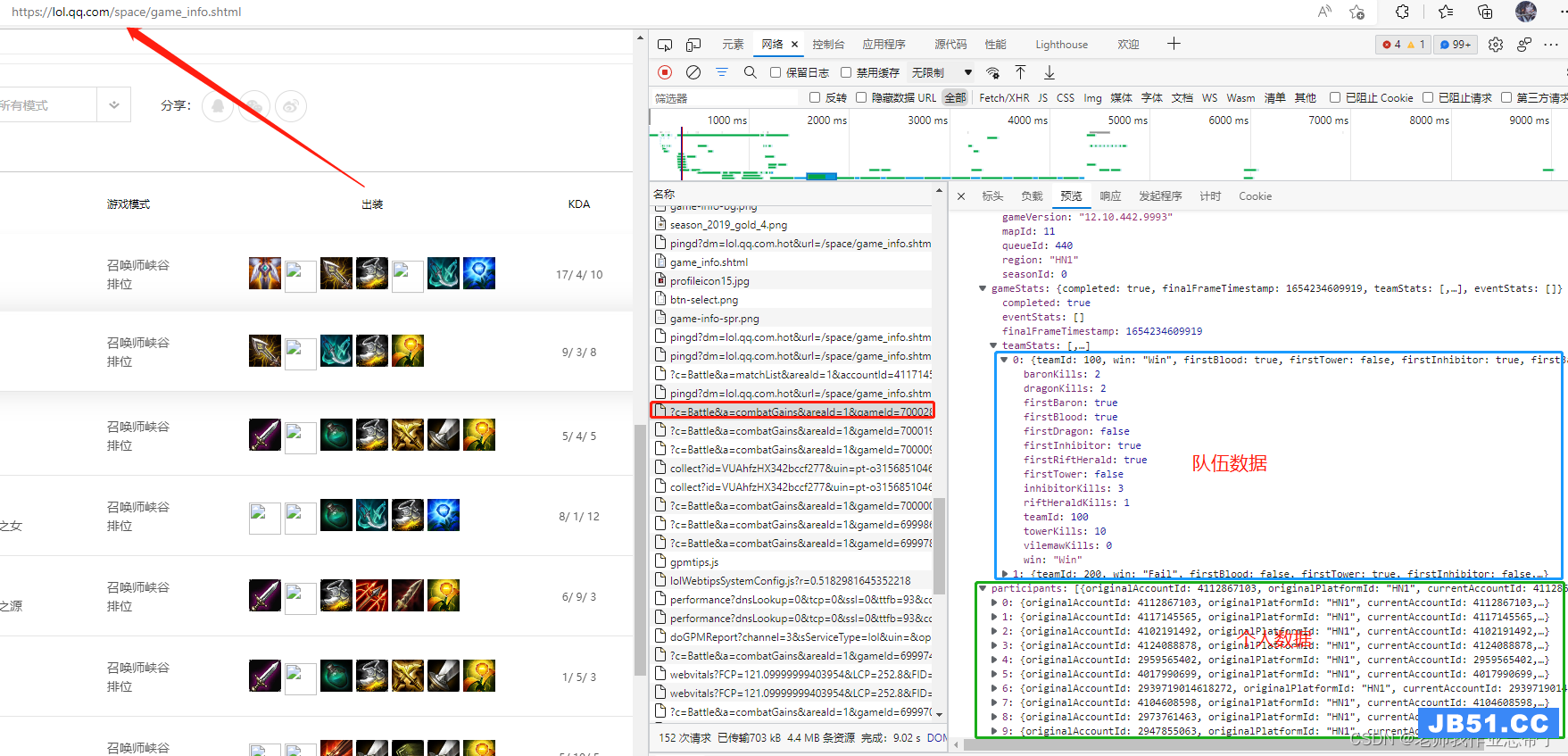
过程虽然有些麻烦但还算简单，感兴趣的可以自己爬一下(注：国内官网 和 opgg 返回的信息各有优缺点，不怕麻烦的建议使用opgg爬取外服某玩家战绩每个event一点点累加，比如我之前就是以大飞老师“hide on bush”为例，局数多也是韩服千分王者质量局。) 

也可以使用现成的：League of Legends Diamond Ranked Games (10 min) | Kaggle

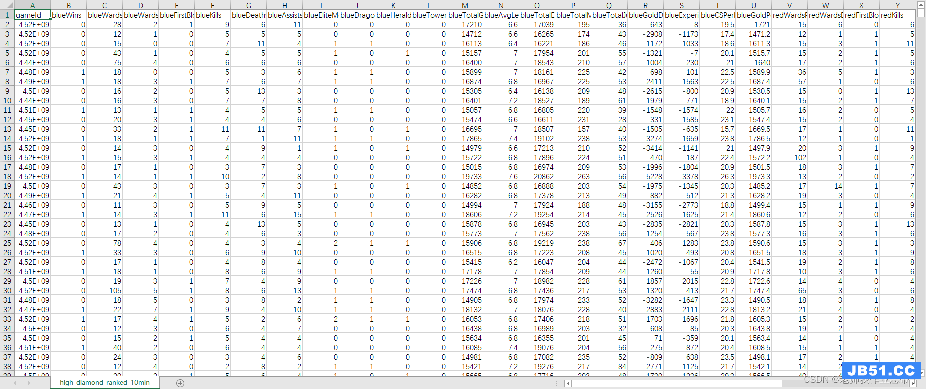
这里一共包含了9879场钻一到大师段位的单双排对局，对局双方几乎是同一水平。每条数据是前10分钟的对局情况，每支队伍有19个特征，红蓝双方共38个特征。这些特征包括英雄击杀、死亡，视野、金钱、经验、等级情况等等。

 

第二步：数据处理

导入工具包

import numpy as np
import pandas as pd
from collections import Counter
from sklearn.model_selection import train_test_split,cross_validate # 划分数据集函数
from sklearn.metrics import accuracy_score # 准确率函数
RANDOM_SEED = 2020 # 固定随机种子

读入数据

csv_data = './data/high_diamond_ranked_10min.csv' # 数据路径
data_df = pd.read_csv(csv_data,sep=',') # 读入csv文件为pandas的DataFrame
data_df = data_df.drop(columns='gameId') # 去掉对局ID列

数据概览

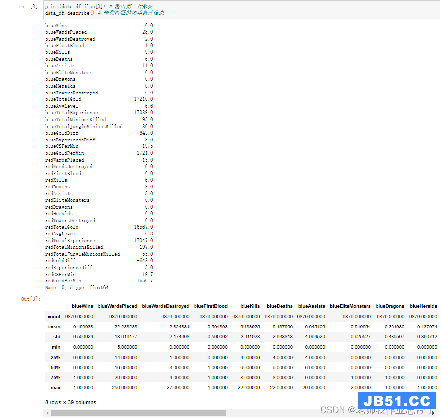
对数据分布有个大致了解，比如我们可以通过.iloc[0]取出数据的第一行并输出。不难看出每个特征都存成了float64浮点数，该对局蓝色方开局10分钟有小优势。同时也可以发现有些特征列是重复冗余的，比如blueGoldDiff表示蓝色队金币优势，redGoldDiff表示红色方金币优势，这两个特征是完全对称的互为相反数，等等。

比如blueKills蓝色方击杀英雄数在前十分钟的平均数是6.14、方差为2.93，中位数是6，百分之五十以上的对局中该特征在4-8之间，等等。

增删特征

除去一些冗杂信息，且像上面说的一般蓝色方击杀等于红色方死亡，或者蓝色与红色方方金币数可以合并为经济差，又或者红色方发生了1血那么蓝色方就没有发生...

drop_features = ['blueGoldDiff','redGoldDiff','blueExperienceDiff','redExperienceDiff','blueCSPerMin','redCSPerMin','blueGoldPerMin','redGoldPerMin'] # 需要舍去的特征列
df = data_df.drop(columns=drop_features) # 舍去特征列
info_names = [c[3:] for c in df.columns if c.startswith('red')] # 取出要作差值的特征名字（除去red前缀）
for info in info_names: # 对于每个特征名字
    df['br' + info] = df['blue' + info] - df['red' + info] # 构造一个新的特征，由蓝色特征减去红色特征，前缀为br
# 其中FirstBlood为首次击杀最多有一只队伍能获得，brFirstBlood=1为蓝，0为没有产生，-1为红
df = df.drop(columns=['blueFirstBlood','redFirstBlood']) # 原有的FirstBlood可删除

经过这一步此时变量df里由原来的38个特征-8(不需要的)+15(红蓝差)-2(一血)，还剩下43个特征值，外加蓝色方是否获胜，一共44列。

特征离散化

决策树ID3算法一般是基于离散特征的，本例中存在很多连续的数值特征，例如队伍金币。直接应用该算法每个值当作一个该特征的一个取值可能造成严重的过拟合，因此需要对特征进行离散化，即将一定范围内的值映射成一个值，例如对用户年龄特征，将0-10映射到0，11-18映射到1，19-25映射到2，25-30映射到3，等等类似，然后在决策树构建时使用映射后的值计算信息增益。

DISCRETE_N = 10
discrete_df = df.copy()
for c in df.columns[1:]: 
    if len(df[c].unique()) <= DISCRETE_N: 
        continue
    else:
        discrete_df[c] = pd.qcut(df[c],DISCRETE_N,precision=0,labels=False,duplicates='drop')

注： 有些特征本身取值就很少，可以跳过离散化。

数据集准备

随机取一部分如20%作测试集，剩下作训练集。sklearn提供了相关工具函数train_test_split。sklearn的输入输出一般为numpy的array矩阵，需要先将pandas的DataFrame取出为numpy的array矩阵。

all_y = discrete_df['blueWins'].values # 所有标签数据
feature_names = discrete_df.columns[1:] # 所有特征的名称
all_x = discrete_df[feature_names].values # 所有原始特征值
# 划分训练集和测试集
x_train,x_test,y_train,y_test = train_test_split(all_x,all_y,test_size=0.2,random_state=RANDOM_SEED)

# ((9879,),(9879,43),(7903,(1976,))

 

第三步：决策树模型的实现

删删改改了很多次，路漫漫其修远~

# 定义决策树类
class DecisionTree(object):
    def __init__(self,classes,features,max_depth=10,min_samples_split=10,impurity_t='entropy'):
        '''
        传入一些可能用到的模型参数，也可能不会用到
        classes表示模型分类总共有几类
        features是每个特征的名字，也方便查询总的共特征数
        max_depth表示构建决策树时的最大深度
        min_samples_split表示构建决策树分裂节点时，如果到达该节点的样本数小于该值则不再分裂
        impurity_t表示计算混杂度（不纯度）的计算方式，例如entropy或gini
        '''
        self.classes = classes
        self.features = features
        self.max_depth = max_depth
        self.min_samples_split = min_samples_split
        self.impurity_t = impurity_t
        self.root = None  # 定义根节点，未训练时为空

    def impurity(self,data):
        '''
        计算某个特征下的信息增益
        :param data: ，numpy一维数组
        :return: 混杂度
        '''
        cnt = Counter(data)  # 计数每个值出现的次数
        probability_lst = [1.0 * cnt[i] / len(data) for i in cnt]
        if self.impurity_t == 'entropy':  # 如果是信息熵
            return -np.sum([p * np.log2(p) for p in probability_lst if p > 0]),cnt  # 返回熵 和可能用到的数据次数(方便以后使用)
        return 1 - np.sum([p * p for p in probability_lst]),cnt  # 否则返回gini系数

    def gain(self,feature,label):
        '''
        计算某个特征下的信息增益
        :param feature: 特征的值，numpy一维数组
        :param label: 对应的标签，numpy一维数组
        :return: 信息增益
        '''
        c_impurity,_ = self.impurity(label)  # 不考虑特征时标签的混杂度

        # 记录特征的每种取值所对应的数组下标
        f_index = {}
        for idx,v in enumerate(feature):
            if v not in f_index:
                f_index[v] = []
            f_index[v].append(idx)

        # 计算根据该特征分裂后的不纯度，根据特征的每种值的数目加权和
        f_impurity = 0
        for v in f_index:
            # 根据该特征取值对应的数组下标 取出对应的标签列表 比如分支1有多少个正负例 分支2有...
            f_l = label[f_index[v]]
            f_impurity += self.impurity(f_l)[0] * len(f_l) / len(label)  # 循环结束得到各分支混杂度的期望

        gain = c_impurity - f_impurity  # 得到gain

        # 有些特征取值很多，天然不纯度高、信息增益高，模型会偏向于取值很多的特征比如日期，但很可能过拟合
        # 计算信息增益率可以缓解该问题
        splitInformation = self.impurity(feature)[0]  # 计算该特征在标签无关时的不纯度
        gainRatio = gain / splitInformation if splitInformation > 0 else gain  # 除数不为0时为信息增益率
        return gainRatio,f_index  # 返回信息增益率，以及每个特征取值的数组下标(方便以后使用)

    def expand_node(self,label,depth,skip_features=set()):
        '''
        递归函数分裂节点
        :param feature:二维numpy（n*m）数组，每行表示一个样本，n行，有m个特征
        :param label:一维numpy（n）数组，表示每个样本的分类标签
        :param depth:当前节点的深度
        :param skip_features:表示当前路径已经用到的特征
        在当前ID3算法离散特征的实现下，一条路径上已经用过的特征不会再用（其他实现有可能会选重复特征）
        '''

        l_cnt = Counter(label)  # 计数每个类别的样本出现次数
        if len(l_cnt) <= 1:  # 如果只有一种类别了，无需分裂，已经是叶节点
            return label[0]  # 只需记录类别
        if len(label) < self.min_samples_split or depth > self.max_depth:  # 如果达到了最小分裂的样本数或者最大深度的阈值
            return l_cnt.most_common(1)[0][0]  # 则只记录当前样本中最多的类别

        f_idx,max_gain,f_v_index = -1,-1,None  # 准备挑选分裂特征
        for idx in range(len(self.features)):  # 遍历所有特征
            if idx in skip_features:  # 如果当前路径已经用到，不用再算
                continue
            f_gain,fv = self.gain(feature[:,idx],label)  # 计算特征的信息增益，fv是特征每个取值的样本下标

            # if f_gain <= 0: # 如果信息增益不为正，跳过该特征
            #   continue
            if f_idx < 0 or f_gain > max_gain:  # 如果个更好的分裂特征
                f_idx,f_v_index = idx,f_gain,fv  # 则记录该特征

            # if f_idx < 0: # 如果没有找到合适的特征，即所有特征都没有信息增益
            #   return l_cnt.most_common(1)[0][0] # 则只记录当前样本中最多的类别

        decision = {}  # 用字典记录每个特征取值所对应的子节点，key是特征取值，value是子节点
        skip_features = set([f_idx] + [f for f in skip_features])  # 子节点要跳过的特征包括当前选择的特征
        for v in f_v_index:  # 遍历特征的每种取值
            decision[v] = self.expand_node(feature[f_v_index[v],:],label[f_v_index[v]],# 取出该特征取值所对应的样本
                                           depth=depth + 1,skip_features=skip_features)  # 深度+1，递归调用节点分裂
        # 返回一个元组，有三个元素
        # 第一个是选择的特征下标，第二个特征取值和对应的子节点(字典)，第三个是到达当前节点的样本中最多的类别
        return (f_idx,decision,l_cnt.most_common(1)[0][0])

    def traverse_node(self,node,feature):
        '''
        预测样本时从根节点开始遍历节点，根据特征路由。
        :param node: 当前到达的节点，例如self.root
        :param feature: 长度为m的numpy一维数组
        '''
        assert len(self.features) == len(feature)  # 要求输入样本特征数和模型定义时特征数目一致
        if type(node) is not tuple:  # 如果到达了一个节点是叶节点（不再分裂），则返回该节点类别
            return node
        fv = feature[node[0]]  # 否则取出该节点对应的特征值，node[0]记录了特征的下标
        if fv in node[1]:  # 根据特征值找到子节点，注意需要判断训练节点分裂时到达该节点的样本是否有该特征值（分支）
            return self.traverse_node(node[1][fv],feature)  # 如果有，则进入到子节点继续遍历
        return node[-1]  # 如果没有，返回训练时到达当前节点的样本中最多的类别

    def fit(self,label):
        '''
        训练模型
        :param feature:feature为二维numpy（n*m）数组，每行表示一个样本，有m个特征
        :param label:label为一维numpy（n）数组，表示每个样本的分类标签
        '''
        assert len(self.features) == len(feature[0])  # 输入数据的特征数目应该和模型定义时的特征数目相同
        self.root = self.expand_node(feature,depth=1)  # 从根节点开始分裂，模型记录根节点

    def predict(self,feature):
        '''
        预测
        :param feature:输入feature可以是一个一维numpy数组也可以是一个二维numpy数组
        如果是一维numpy（m）数组则是一个样本，包含m个特征，返回一个类别值
        如果是二维numpy（n*m）数组则表示n个样本，每个样本包含m个特征，返回一个numpy一维数组
        '''
        assert len(feature.shape) == 1 or len(feature.shape) == 2  # 只能是1维或2维
        if len(feature.shape) == 1:  # 如果是一个样本
            return self.traverse_node(self.root,feature)  # 从根节点开始路由
        return np.array([self.traverse_node(self.root,f) for f in feature])  # 如果是很多个样本

    def get_params(self,deep):  # 要调用sklearn的cross_validate需要实现该函数返回所有参数
        return {'classes': self.classes,'features': self.features,'max_depth': self.max_depth,'min_samples_split': self.min_samples_split,'impurity_t': self.impurity_t}

    def set_params(self,**parameters):  # 要调用sklearn的GridSearchCV需要实现该函数给类设定所有参数
        for parameter,value in parameters.items():
            setattr(self,parameter,value)
        return self


# 定义决策树模型，传入算法参数
DT = DecisionTree(classes=[0,1],features=feature_names,max_depth=5,impurity_t='gini')

DT.fit(x_train,y_train)  # 在训练集上训练
p_test = DT.predict(x_test)  # 在测试集上预测，获得预测值
print(p_test)  # 输出预测值
test_acc = accuracy_score(p_test,y_test)  # 将测试预测值与测试集标签对比获得准确率
print('accuracy: {:.4f}'.format(test_acc))  # 输出准确率

[0 1 0 ... 0 1 1]
accuracy: 0.6964

此时的准确率为0.6964，下面我们进行模型调优。

 

第四步：模型调优

在测试集上对不同的混杂度计算方式、深度、最小分裂阈值进行五折交叉验证。

%%time

best = None # 记录最佳结果
for impurity_t in ['entropy','gini']: # 遍历不纯度的计算方式
    for max_depth in range(1,6): # 遍历最大树深度
        for min_samples_split in [50,100,200,500,1000]: # 遍历节点分裂最小样本数的阈值
            DT = DecisionTree(classes=[0,# 定义决策树
                              max_depth=max_depth,min_samples_split=min_samples_split,impurity_t=impurity_t)
            cv_result = cross_validate(DT,x_train,scoring=('accuracy'),cv=5) # 5折交叉验证            
            cv_acc = np.mean(cv_result['test_score']) # 5折平均准确率
            current = (cv_acc,max_depth,min_samples_split,impurity_t) # 记录参数和结果
            if best is None or cv_acc > best[0]: # 如果是比当前最佳更好的结果
                best = current # 记录最好结果
                print('better cv_accuracy: {:.4f},max_depth={},min_samples_split={},impurity_t={}'.format(*best)) # 输出准确率和参数
            else:
                print('cv_accuracy: {:.4f},impurity_t={}'.format(*current)) # 输出准确率和参数

DT = DecisionTree(classes=[0,max_depth=best[1],min_samples_split=best[2],impurity_t=best[3])  # 取最佳参数
DT.fit(x_train,y_train) # 在训练集上训练
p_test = DT.predict(x_test) # 在测试集上预测，获得预测值
print(p_test) # 输出预测值
test_acc = accuracy_score(p_test,y_test) # 将测试预测值与测试集标签对比获得准确率
print('accuracy: {:.4f}'.format(test_acc)) # 输出准确率

better cv_accuracy: 0.7257,max_depth=1,min_samples_split=50,impurity_t=entropy
cv_accuracy: 0.7257,min_samples_split=100,min_samples_split=200,min_samples_split=500,min_samples_split=1000,impurity_t=entropy
cv_accuracy: 0.7254,max_depth=2,impurity_t=entropy
better cv_accuracy: 0.7267,max_depth=3,impurity_t=entropy
better cv_accuracy: 0.7272,impurity_t=entropy
better cv_accuracy: 0.7281,impurity_t=entropy
better cv_accuracy: 0.7286,impurity_t=entropy
cv_accuracy: 0.7237,max_depth=4,impurity_t=entropy
cv_accuracy: 0.7252,impurity_t=entropy
cv_accuracy: 0.7285,impurity_t=entropy
better cv_accuracy: 0.7290,impurity_t=entropy
cv_accuracy: 0.7257,impurity_t=entropy
cv_accuracy: 0.7149,impurity_t=entropy
cv_accuracy: 0.7210,impurity_t=entropy
cv_accuracy: 0.7290,impurity_t=gini
cv_accuracy: 0.7257,impurity_t=gini
cv_accuracy: 0.7255,impurity_t=gini
cv_accuracy: 0.7218,impurity_t=gini
cv_accuracy: 0.7235,impurity_t=gini
cv_accuracy: 0.7250,impurity_t=gini
cv_accuracy: 0.7174,impurity_t=gini
cv_accuracy: 0.7248,impurity_t=gini
cv_accuracy: 0.7261,impurity_t=gini
cv_accuracy: 0.7259,impurity_t=gini
cv_accuracy: 0.7076,impurity_t=gini
cv_accuracy: 0.7185,impurity_t=gini
cv_accuracy: 0.7207,impurity_t=gini

使用max_depth=4,impurity_t=entropy在训练集上进行训练，并在测试集上预测，将测试预测值与测试集标签对比获得准确率：显然提升了。

[0 1 0 ... 0 1 1]

accuracy: 0.7171

Wall time: 1min 19s

也可以调用sklearn的GridSearchCV自动且多线程搜索参数，和上面的流程类似。

%%time

parameters = {'impurity_t':['entropy','gini'],'max_depth': range(1,6),'min_samples_split': [50,1000]} # 定义需要遍历的参数
DT = DecisionTree(classes=[0,features=feature_names) # 定义决策树，可以不传参数，由GridSearchCV传入构建
grid_search = GridSearchCV(DT,parameters,scoring='accuracy',cv=5,verbose=100,n_jobs=4) # 传入模型和要遍历的参数
grid_search.fit(x_train,y_train) # 在所有数据上搜索参数
print(grid_search.best_score_,grid_search.best_params_) # 输出最佳指标和最佳参数

DT = DecisionTree(classes=[0,**grid_search.best_params_)  # 取最佳参数
DT.fit(x_train,y_test) # 将测试预测值与测试集标签对比获得准确率
print('accuracy: {:.4f}'.format(test_acc)) # 输出准确率

Fitting 5 folds for each of 50 candidates,totalling 250 fits
0.7289642831407777 {'impurity_t': 'entropy','max_depth': 4,'min_samples_split': 500}
[0 1 0 ... 0 1 1]
accuracy: 0.7171
Wall time: 24.6 s

查看节点的特征

best_dt = grid_search.best_estimator_ # 取出最佳模型
print('root',best_dt.features[best_dt.root[0]]) # 输出根节点特征

root brTotalGold

可见前10分钟最能影响胜率的是红蓝双方的经济差 

for fv in best_dt.root[1]: # 遍历根节点的每种特征取值
    print(fv,'->',best_dt.features[best_dt.root[1][fv][0]],'-> ...') # 输出下一层特征

9 -> redDragons -> ...
1 -> blueTowersDestroyed -> ...
3 -> redEliteMonsters -> ...
5 -> redTowersDestroyed -> ...
2 -> blueTowersDestroyed -> ...
4 -> brTowersDestroyed -> ...
7 -> redEliteMonsters -> ...
8 -> brTowersDestroyed -> ...
0 -> brKills -> ...
6 -> brTowersDestroyed -> ...

根节点这个特征对应取值0-9(我们之前对金币进行了离散化)所对应的下一层的特征...

       

ps:这个其实来自于我们定义的 expand_node 函数返回值，

return (f_idx,l_cnt.most_common(1)[0][0]) ，

第一个是选择的特征下标，第二个特征取值和对应的子节点(字典)，第三个是到达当前节点的样本中最多的类别。

它的形状/结果其实是这样的：

(38,{9: (20,{0: (23,{1: 1,2: 1,4: 1,0: 1,3: 1,5: 1,6: 1,7: 1,8: 1},1),1: 1},1: (8,{0: (7,{0: (20,{1: 0,0: 0},0),1: 0},3: (19,{0: 0,1: 0,2: 0},5: (22,{0: (19,{0: 1,2: 0,1: 1,2: 1},2: (8,{0: (22,{0: (6,4: (37,{0: (8,{0: (5,-1: 0,7: (19,8: (37,0: (31,4: 0,3: 0},6: (37,0: 1},-1: 0},1)},0)